Transform Data

Of the 10,000 sightings, 4,465 carry a depth — and the deepest of them comes from 4,838 meters down. The sightings table already says that much; what it will not say is which octopus that was or where in any human sense, because it names species by a numeric ID and locations as raw coordinates. This step joins occurrences, species, depth_zones and basins with SQL into one 10,000-row atlas that turns IDs into names and places every sighting in its ocean — and, where a depth was recorded, its depth zone — and it introduces the mapping model that keeps your source data safe while you do it. Step 3 of the Getting Started arc.

Two ways to do it — pick a tab in Set it up below. Doing it with Kai, the run is part of the prompt — you only check the result. Doing it yourself, you run it afterwards in the section below the tabs.

What you need

Four tables in Storage — occurrences, species, depth_zones and basins — from Get Your Data In. They sit in whatever bucket the connector created, and its name contains a configuration ID, so yours will not match the screenshots.

That does not matter. What the SQL depends on is the Table name you give each table in the input mapping below: those must be exactly occurrences, species, depth_zones and basins, or you have to edit the queries to match.

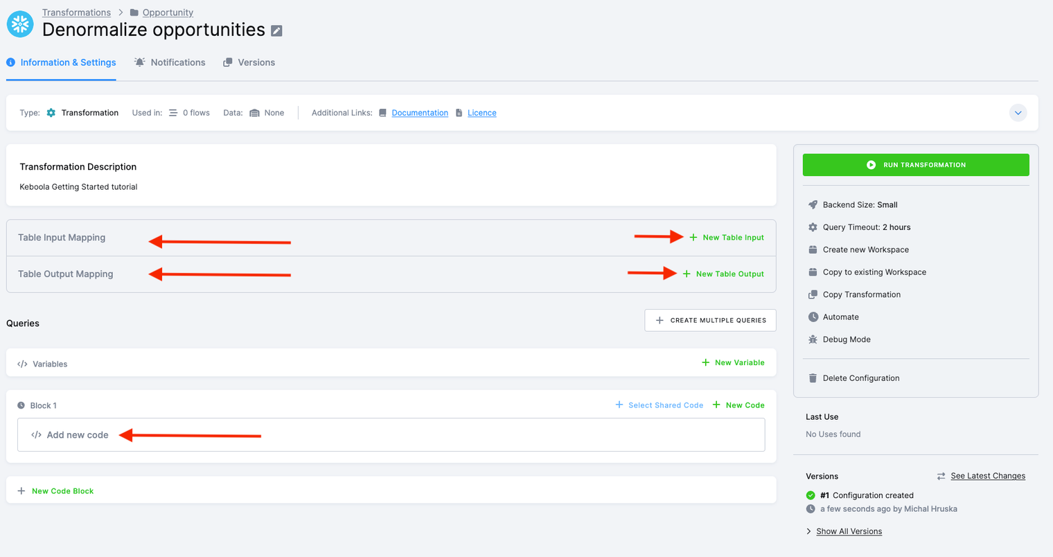
How a transformation works

A transformation never runs against your Storage tables directly. Keboola copies the tables you ask for into a temporary database schema, runs your queries there, and copies back only the results you ask for. Three settings control that:

1. Input mapping — which Storage tables get copied in, and what they are called inside the transformation. Anything you do not list is not visible to your code.
2. Output mapping — which tables your code produces get written back to Storage, and where. Anything you do not list is thrown away when the job ends.
3. Queries — the SQL itself, organized into named code blocks.

That is the safeguard: the only tables your transformation can change are the ones named in the output mapping. It is also what lets Keboola track data lineage across the project.

Set it up

Do it with Kai

Writing SQL transformations is Kai’s home ground (SQL Transformations), and it already has your table schemas in front of it. Open Kai Agent in the top bar and ask:

Create a SQL transformation called "Octopus atlas" writing to out.c-octopus-atlas.octopus_atlas.
Start from every column of occurrences with latitude, longitude and depth_m cast to numbers.
Join species on aphia_id, adding scientific_name, family, and a display_name that falls back to
the scientific name when common_name is empty. Add depth_zones.zone_name as depth_zone by depth
range (left join — many sightings have no depth). Add basins.basin by latitude and longitude
range; use half-open ranges (>= min and < max) so boundary points match exactly one basin.
Outline the approach first, then build it and run it.

Spelling out the derived columns is the point — ask only for “a map table” and you will get a different set, and the check below will not match. The half-open-ranges sentence matters most: with BETWEEN, a sighting sitting exactly on a basin boundary lands in two basins and the row count comes out above 10,000. Asking for the outline first is worth it too: you get to read the joins before they run. One difference from the hand-built version: Kai builds the transformation on read-only input, so you will not see an input mapping in its configuration — the mapping sections on this page describe the hand-built path.

Check: 10,000 rows, 12 columns — the original 7 plus the five named in Run it and check the result, below the tabs. If the count differs, the joins differ: re-prompt, or fix the code in place. Later steps only depend on the table name, so a close-enough table is fine.

Do it yourself

Create the transformation

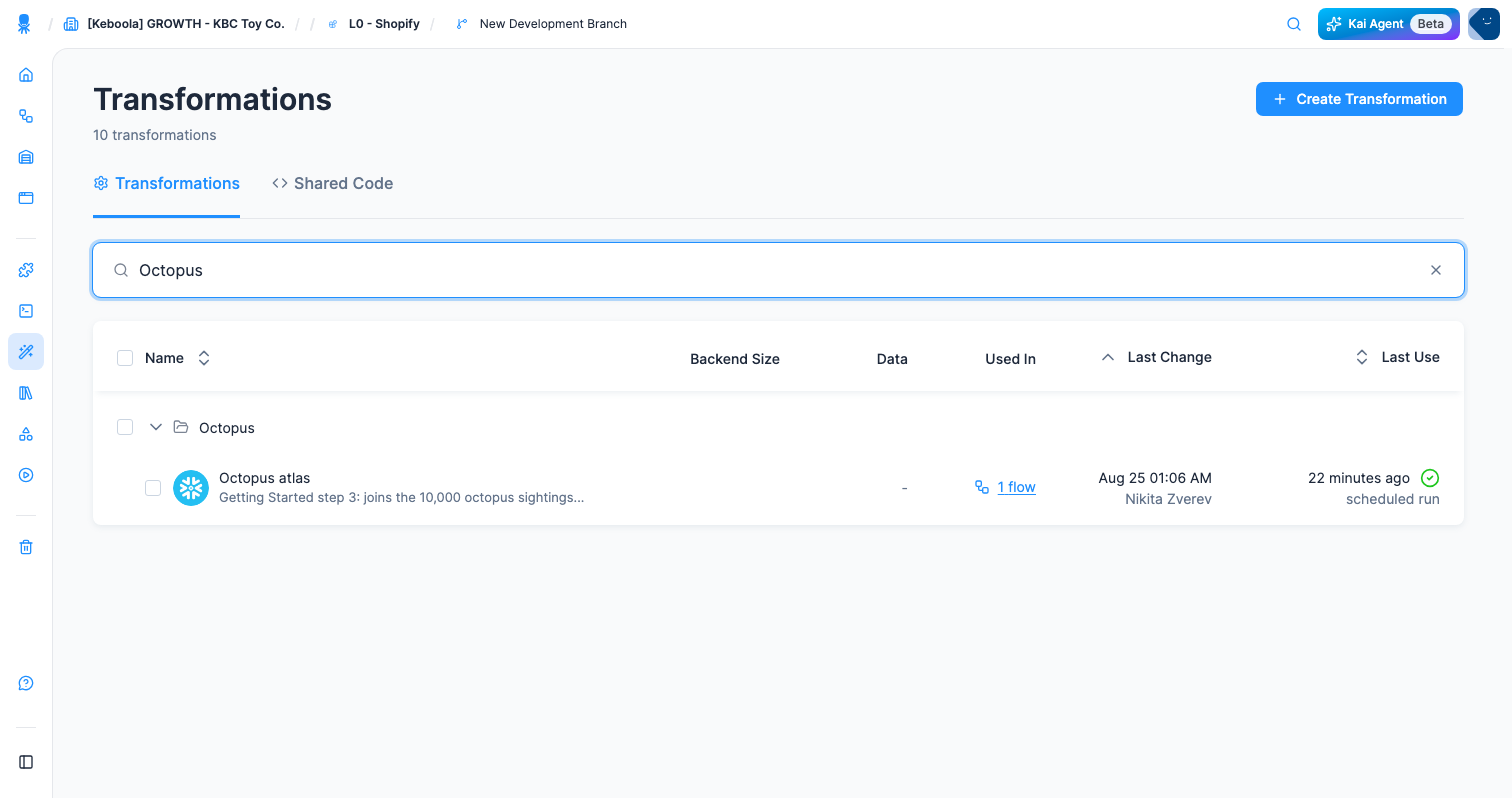
1. Open Transformations.

   

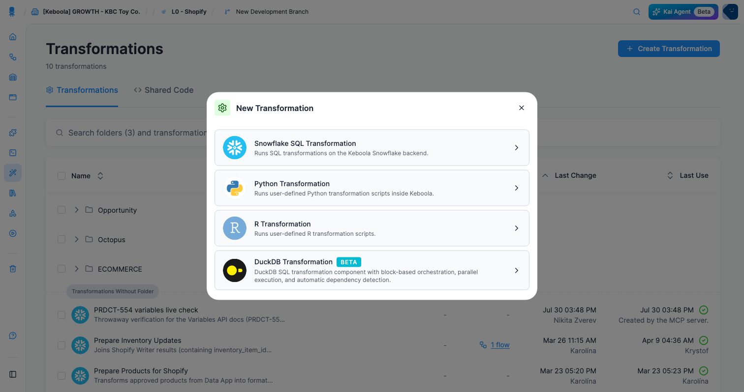
2. Click Create Transformation. The New Transformation dialog lists what this project can run, and it differs by project: an SQL entry for your backend — Snowflake SQL Transformation or Google BigQuery Transformation — plus Python, R, DuckDB (Beta), and on some projects dbt Core. Take the dialog as the authority on your project rather than this sentence.

   This list is how you find out which SQL dialect you need. New Free Plan projects default to the BigQuery backend; contract customers choose theirs. Pick the SQL transformation your project offers, and use the matching query block below.

   

3. Name it Octopus atlas, add a description, and in Folder type Octopus and pick Create folder “Octopus”. Folders are cosmetic, but they are the difference between a browsable project and a wall of configurations. If the dialog offers Use predefined code pattern, ignore it. Click Create transformation.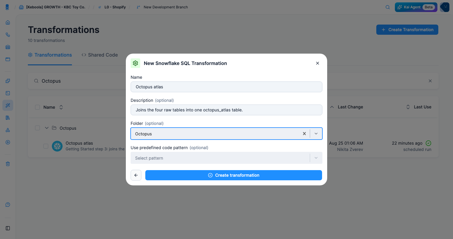

   

Set the input mapping

1. In Table Input Mapping, click Add Table Input.

2. Source searches your Storage as you type. Type occurrences and tick the table; the picker is multi-select, so tick species, depth_zones and basins too — it keeps a count of what you have chosen.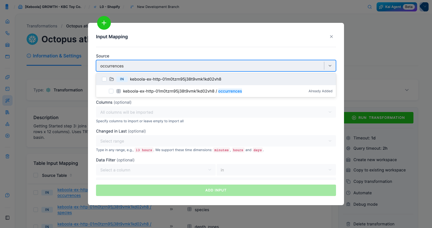

   

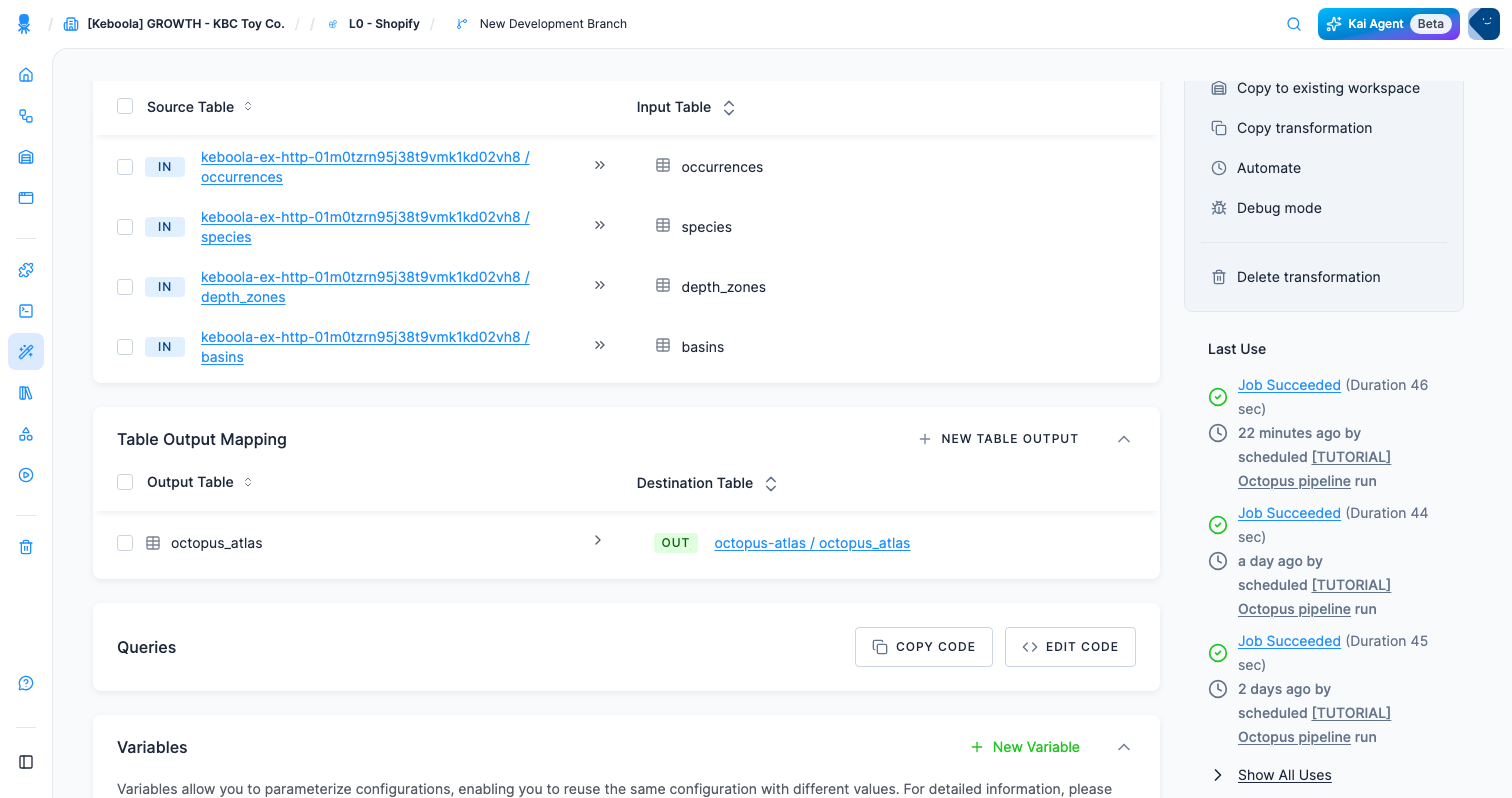
3. Click Add Input. Each table arrives with its Input Table name taken from the source table — occurrences, species, depth_zones, basins.

   Those four names are what your SQL uses, which is why the queries below work no matter which bucket the tables actually live in. If you add a table on its own rather than in a batch, the dialog exposes the same value as a Table name field you can edit.

You should end up with four inputs, listed as Source Table → Input Table:

Input mapping has more to it — incremental processing with Changed in Last, column filters, data filters. None of it is needed here; see input mapping when you have a large table to process.

Set the output mapping

1. In Table Output Mapping, click New Table Output.

   Output mapping opens in Guided Mode — the standard, copy-based mapping the steps below describe. If your project also shows Direct Mode, ignore it here: that writes straight to Storage and is a private beta.

2. Name the table octopus_atlas. This is the name of a table your SQL will create — it does not exist yet. The field is labelled Table name, or Which table should we save? in Guided Mode. If the dialog warns you about case-sensitivity and suggests an UPPERCASE name, ignore the suggestion here and match your SQL exactly: the query blocks below create octopus_atlas in lower case, and the name has to be the one the query actually creates.

3. Destination is filled in for you from the transformation’s name: out.c-octopus-atlas.octopus_atlas — the out stage, a bucket named after the transformation, and the table. Neither the bucket nor the table exists yet; both are created the first time the transformation runs.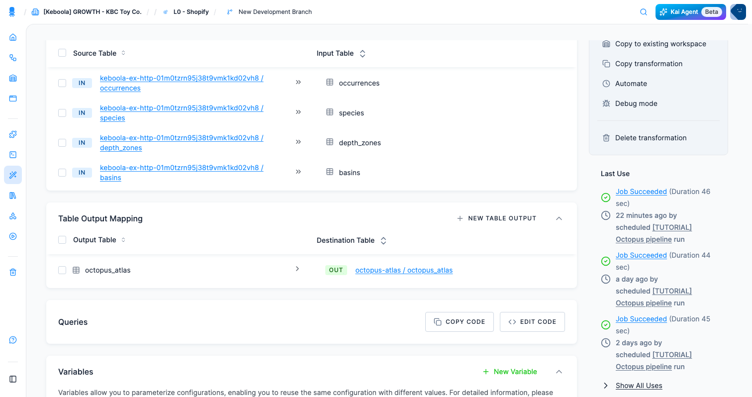

   

Write the queries

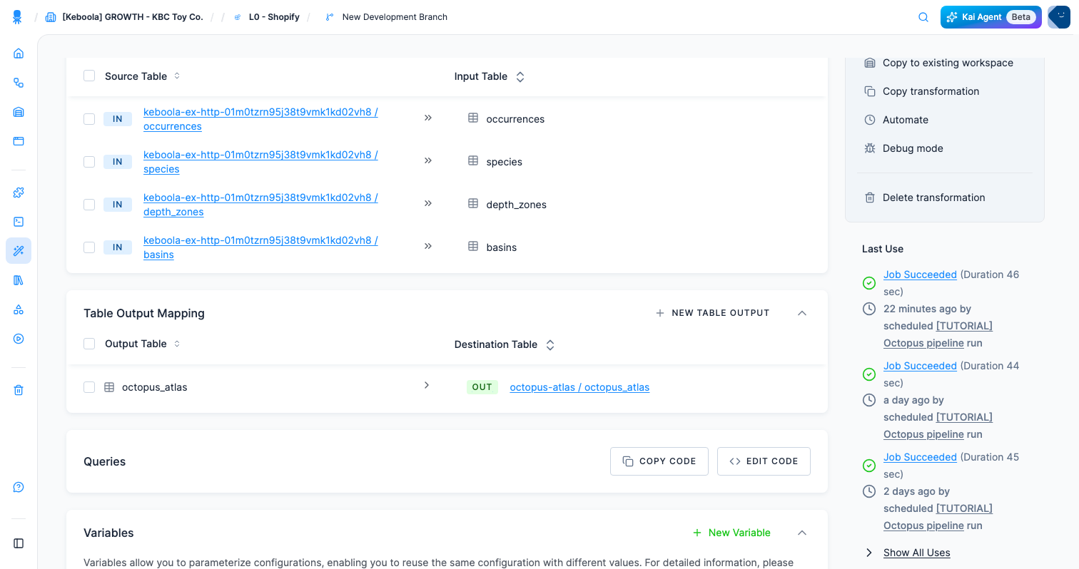
In the empty Queries section, click Create Multiple Queries. Your SQL lives in a code inside a block: you get Block 1 holding one code. Paste the SQL for your project’s backend and save.

You may get an editor for that one code, where you can also name it — call it Octopus atlas. You may instead get a single All Queries editor holding every block and code at once, with the structure marked by comment lines like /* ===== BLOCK: Block 1 ===== */; there, replace the -- Your code goes here line and leave those markers alone, since they are what keeps the blocks apart.

Later you can add another code to the same block with New Code, or a whole second block with New Code Block — that is how a longer transformation gets organized. Once there is code, the Queries header offers Copy Code and Edit Code.

If your project uses Snowflake

CREATE TABLE "tmp_occurrences" AS
    SELECT "occurrence_id", "aphia_id",
        TRY_TO_DOUBLE("latitude")  AS "latitude",
        TRY_TO_DOUBLE("longitude") AS "longitude",
        TRY_TO_DOUBLE("depth_m")   AS "depth_m",
        "year", "event_date"
    FROM "occurrences";

CREATE TABLE "tmp_basins" AS
    SELECT "basin",
        TRY_TO_DOUBLE("min_lat") AS "min_lat", TRY_TO_DOUBLE("max_lat") AS "max_lat",
        TRY_TO_DOUBLE("min_lon") AS "min_lon", TRY_TO_DOUBLE("max_lon") AS "max_lon"
    FROM "basins";

CREATE TABLE "tmp_zones" AS
    SELECT "zone_name",
        TRY_TO_DOUBLE("min_depth_m") AS "min_depth_m",
        TRY_TO_DOUBLE("max_depth_m") AS "max_depth_m"
    FROM "depth_zones";

CREATE TABLE "octopus_atlas" AS
    SELECT "tmp_occurrences".*,
        "species"."scientific_name",
        "species"."family",
        COALESCE(NULLIF("species"."common_name", ''), "species"."scientific_name") AS "display_name",
        "tmp_zones"."zone_name" AS "depth_zone",
        "tmp_basins"."basin"
    FROM "tmp_occurrences"
        JOIN "species"
            ON "tmp_occurrences"."aphia_id" = "species"."aphia_id"
        JOIN "tmp_basins"
            ON "tmp_occurrences"."latitude"  >= "tmp_basins"."min_lat"
           AND "tmp_occurrences"."latitude"  <  "tmp_basins"."max_lat"
           AND "tmp_occurrences"."longitude" >= "tmp_basins"."min_lon"
           AND "tmp_occurrences"."longitude" <  "tmp_basins"."max_lon"
        LEFT JOIN "tmp_zones"
            ON "tmp_occurrences"."depth_m" >= "tmp_zones"."min_depth_m"
           AND "tmp_occurrences"."depth_m" <  "tmp_zones"."max_depth_m";

Four queries, in order: three that cast the CSV text columns into real numbers — tables loaded from CSV arrive as text, and depth_m is empty on more than half the rows, which is exactly what TRY_TO_DOUBLE turns into a clean NULL — then one join that builds the atlas. Only that last table is in the output mapping, so the three tmp_ tables vanish when the job finishes.

Two join details carry the meaning. The species join is a plain equality, but depth_zone comes from a LEFT JOIN — a sighting without a depth keeps its row and gets a NULL zone rather than disappearing. And both range joins are half-open (>= min AND < max): with BETWEEN, a sighting sitting exactly on a basin boundary would land in two basins and duplicate its row.

Every identifier is double-quoted because Snowflake uppercases unquoted ones.

If your project uses BigQuery

BigQuery does not quote identifiers this way, and CTEs replace the temporary tables. It is written to produce the same table:

CREATE TABLE octopus_atlas AS
WITH tmp_occurrences AS (
    SELECT
        occurrence_id,
        aphia_id,
        SAFE_CAST(latitude AS FLOAT64)  AS latitude,
        SAFE_CAST(longitude AS FLOAT64) AS longitude,
        SAFE_CAST(depth_m AS FLOAT64)   AS depth_m,
        year,
        event_date
    FROM
        occurrences
),
tmp_basins AS (
    SELECT
        basin,
        SAFE_CAST(min_lat AS FLOAT64) AS min_lat,
        SAFE_CAST(max_lat AS FLOAT64) AS max_lat,
        SAFE_CAST(min_lon AS FLOAT64) AS min_lon,
        SAFE_CAST(max_lon AS FLOAT64) AS max_lon
    FROM
        basins
),
tmp_zones AS (
    SELECT
        zone_name,
        SAFE_CAST(min_depth_m AS FLOAT64) AS min_depth_m,
        SAFE_CAST(max_depth_m AS FLOAT64) AS max_depth_m
    FROM
        depth_zones
)
SELECT
    tmp_occurrences.*,
    species.scientific_name,
    species.family,
    COALESCE(NULLIF(species.common_name, ''), species.scientific_name) AS display_name,
    tmp_zones.zone_name AS depth_zone,
    tmp_basins.basin
FROM
    tmp_occurrences
JOIN
    species ON tmp_occurrences.aphia_id = species.aphia_id
JOIN
    tmp_basins ON tmp_occurrences.latitude  >= tmp_basins.min_lat
              AND tmp_occurrences.latitude  <  tmp_basins.max_lat
              AND tmp_occurrences.longitude >= tmp_basins.min_lon
              AND tmp_occurrences.longitude <  tmp_basins.max_lon
LEFT JOIN
    tmp_zones ON tmp_occurrences.depth_m >= tmp_zones.min_depth_m
             AND tmp_occurrences.depth_m <  tmp_zones.max_depth_m;

Run it and check the result

Coming from the Kai tab? The run already happened — the prompt asked for it. Skip to the row-count check below.

Click Run Transformation and confirm with Run. That creates a background job which copies the input tables in, runs your SQL, and writes octopus_atlas back to Storage. The job log spells the mechanism out — “Loading 4 tables to workspace”, then a line per table cloned into the workspace — which is the mapping model from the top of this page, in action.

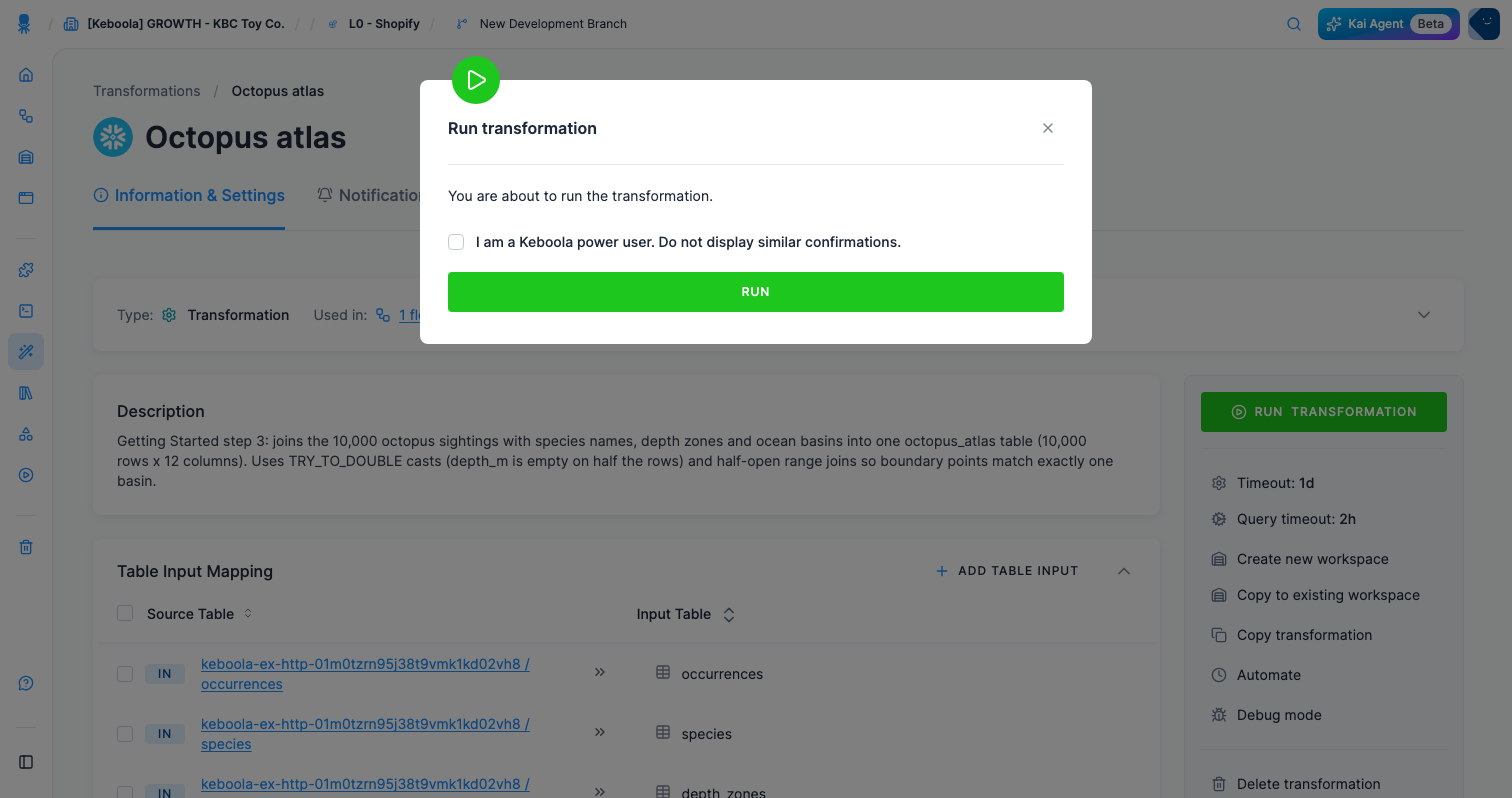
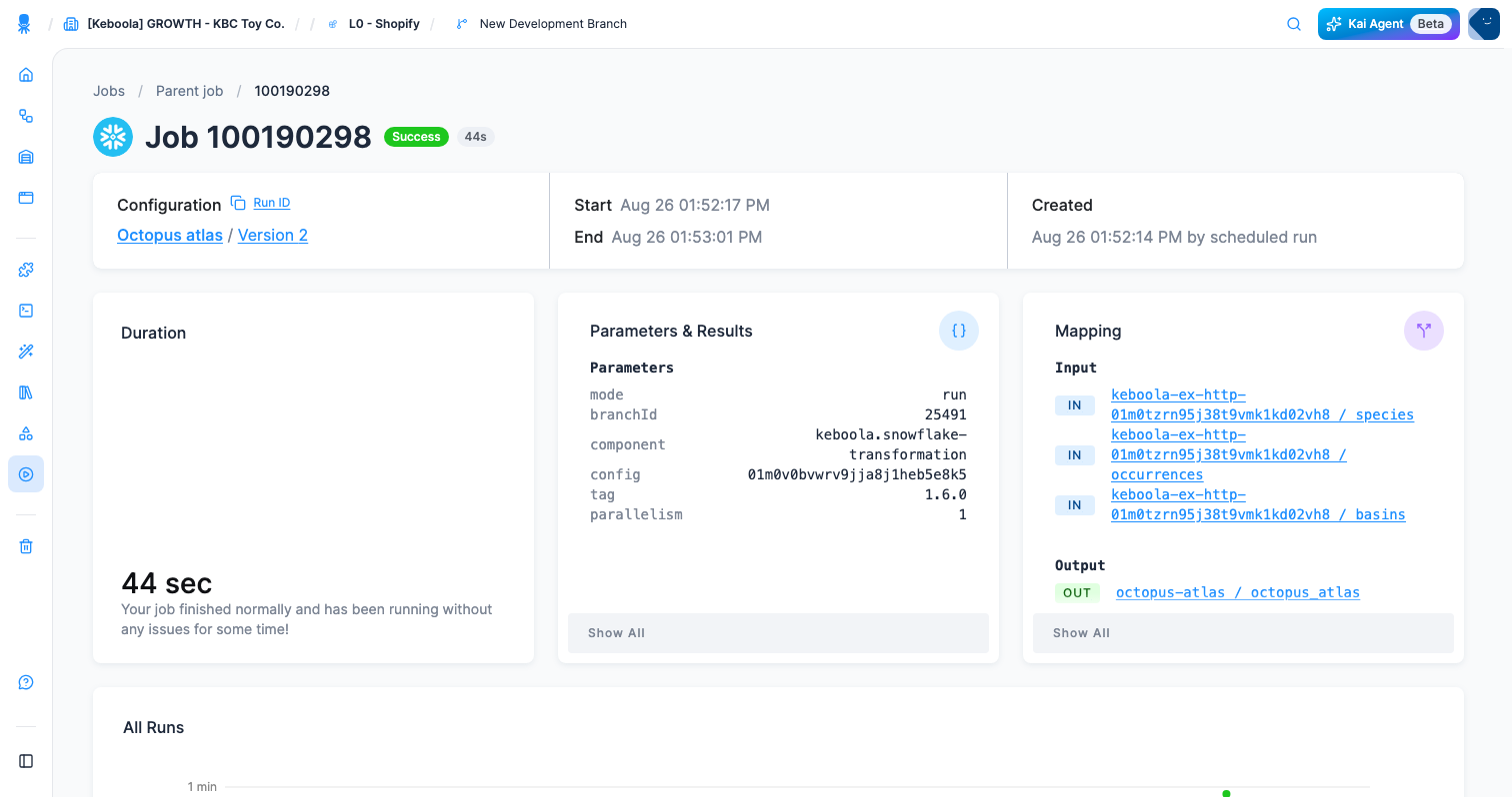
A notification appears with a Show job link — Snowflake SQL job has been scheduled, or your backend’s equivalent — and you can also find it under Jobs. It takes about a minute, and a green Success means it worked.

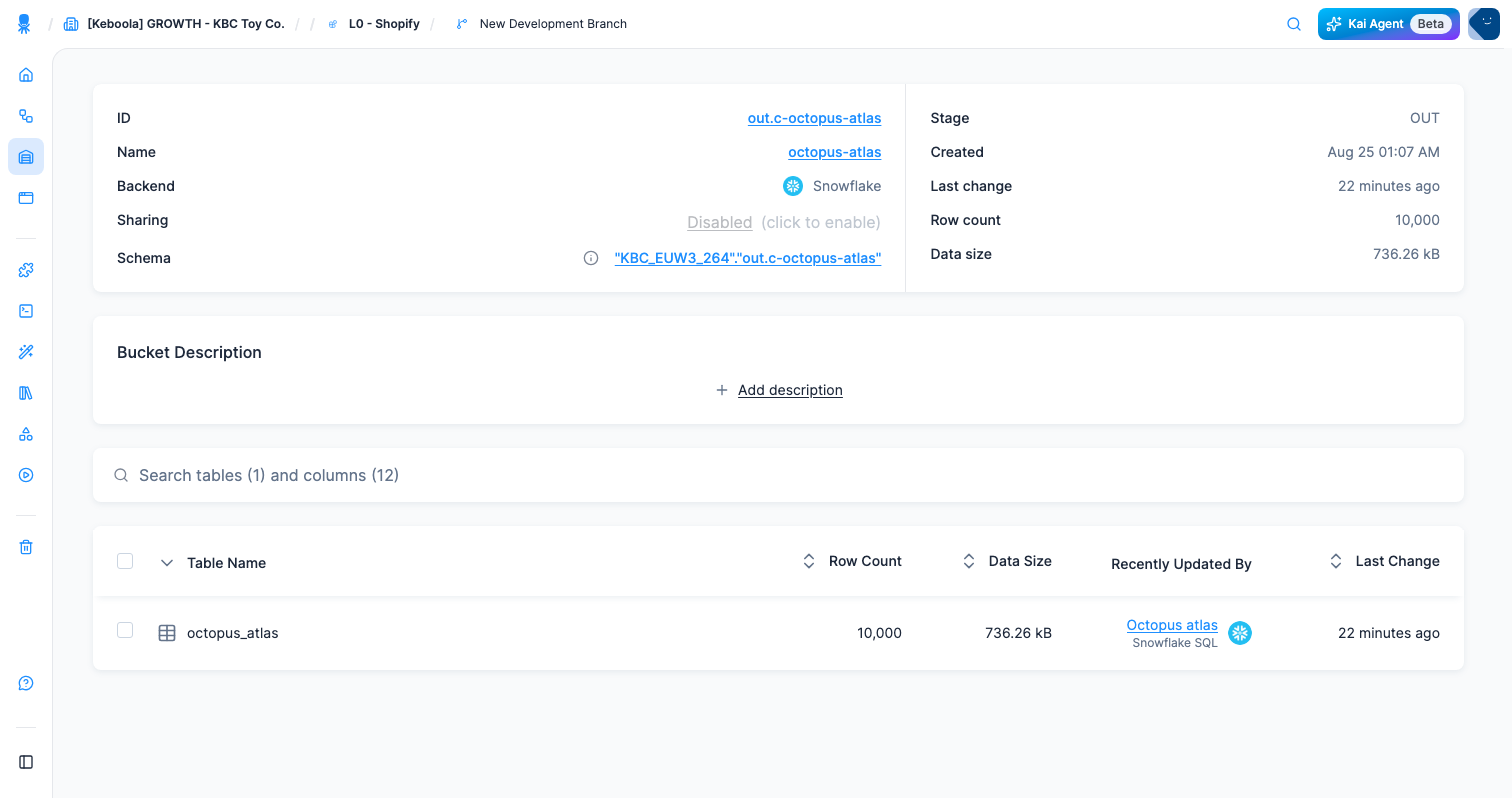
Then open Storage: there is a new bucket out.c-octopus-atlas — listed as octopus-atlas with an OUT badge, the same way the in.c- prefix was hidden in step 2 — holding octopus_atlas — 10,000 rows and 12 columns. That row count is the same as the source occurrences table, which is the quickest sanity check that the joins matched every row without duplicating any: more than 10,000 means a range join double-matched, fewer means an inner join dropped sightings.

The 12 columns are the original 7 plus the five the SQL added: scientific_name, family, display_name, depth_zone and basin. Open the Data Sample tab and the atlas already answers things the raw file could not — sort by depth_m descending and the deepest row is Grimpoteuthis challengeri — a dumbo octopus, though the data only knows its Latin name — recorded at 4,838 meters in the abyssal zone.

The table list also has a Recently Updated By column, naming the transformation and its backend (Octopus atlas / Snowflake SQL here) — the fastest way to answer “where did this table come from?” months later.

Running the transformation again simply rebuilds the table; it is safe to re-run while you are experimenting.

If it goes wrong

• Object 'SPECIES' does not exist (Snowflake). A table is missing from the input mapping, or the Table name inside the transformation differs from what the SQL uses. Snowflake uppercases unquoted identifiers, which is why every identifier is double-quoted. On BigQuery the equivalent error is Table ... was not found.
• The job succeeds but Storage has no new table. The output mapping is empty or names a table your SQL never creates. The names must match exactly: octopus_atlas.
• Numeric value '' is not recognized. Tables loaded from CSV arrive as text columns unless you give them types, so an empty cell is '' rather than NULL — and depth_m is empty on more than half of these rows, which is why the queries cast with TRY_TO_DOUBLE (Snowflake) / SAFE_CAST (BigQuery) before comparing. If you see this error, a cast got dropped somewhere.
• The atlas has more than 10,000 rows. A range join double-matched: a sighting sitting exactly on a boundary fell into two basins or two zones. That happens when BETWEEN (inclusive on both ends) replaces the half-open >= min AND < max the queries use.
• Invalid columns: _timestamp when the output is written. Your input tables were staged by cloning, which copies Keboola’s internal _timestamp column along with the data — and that column cannot be written back to Storage. It is not backend-specific and it is not a problem with the query. The clean fix is the dropTimestampColumn option on the input mapping; see the _timestamp system column. The run behind these screenshots was copy-staged, so the column never appeared.
• You want to see what the query actually returns before saving. That is what a workspace is for.
• You would rather not read the log yourself. Kai has it open already (Troubleshooting): My transformation "Octopus atlas" failed. Read the last job's log and tell me what to fix.

Going further

• Use a Workspace — develop and test queries against a copy of the data before committing them to a transformation. This is how the work is really done.

Next: Send your data somewhere →